Many-to-Many Document Similarity Task
Contents
Many-to-Many Document Similarity Task#
In this section, we implement the traditional LSH appraoch to a hypothetical many-to-many document similarity task. The objective is to bucket similar documents together. The implementation is done through the LSH class which leverages on dask.bag functionality and methods to parallelize the banding technique. Specifically, the map (hash function) and reduce (bucketing) tasks.
The LSH has three main methods:
make_bands- This method takes in the desired number ofbandsas a parameter and returns a dictionary with band labels as keys anddask.bagof (set/document index, signature band) tuples. Here, signature bands are defined as a slice of a document’s signature.Parameters
bands- (int) desired number of bands
Returns
band_dict- (dict) dictionary with band labels as keys and (set/doc index, signature band) tuples as values
get_buckets- This method implementes the map-reduce step of the traditional banding technique. Specifically, signature slices of each band are hashed usinghash_functions(map). The document indices are then grouped according to their hash values.Parameters
hash_functions- (list, default=None) a list of hash functions with size equivalent to the number of bands. A hash function in the list is applied to a band with the same index. When None, the funciton defaults to using the python builtinhashfunction. Note: python’s hash function value for the same input vary across partitions–hence, current implementation stores all elements of a band in one partition.
Returns
band_buckets - (dict) a dictionary with hash bucket as keys and a list of similar document indices as values.
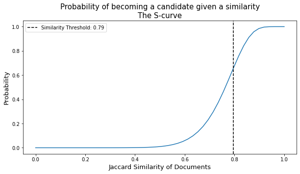
plot_thresh- Shows the S-curve corresponding to the choice of number ofbands. The similirity threshold (i.e., the Jaccard similarity value that is the basis of tagging a pair as candidate pairs or not) is emphasized.Paramters
display_thresh- (bool, default=True) whether to display emphasis on the similarity threshold or not.ax- (matplotlib.pyplot Axis, default=None) axis for plotting.**kwargs- keyword arguments for thematplotlib.pyplot.plot()function.
Returns
matplotlib.pyplotAxis object
Examples#
Here we demonstrate the use of the LSH class on some examples. First off, make sure that a a dask.distributed.Client is initialized since class methods take advantage of the dask.
import numpy as np
import matplotlib.pyplot as plt

from alis.similarity import LSH


from dask.distributed import Client
client = Client()
Example 1#
Suppose a signature matrix with dimensions \((n, m)\)–where \(n\) is the number of documents/sets and \(m\) as the size of each signature vector. Signature vector values are randomly set to be within the 0 to 255 range.
n = 1000 # samples (rows)
m = 100 # signature features (columns)

# signature matrix
signature = np.random.randint(255, size=(n, m))
display(signature)
array([[128,  85, 248, ..., 226,  99,  91],
       [247,  40, 159, ...,  39, 180,  52],
       [161, 150,  16, ..., 138,  26, 230],
       ...,
       [200,  51, 193, ..., 141,  16, 245],
       [ 28, 117,  35, ..., 236, 206, 252],
       [180, 183,  98, ..., 240, 172,  23]])
Running the get_buckets function with compute=False returns a dask.bag which can be inspected further using dask.bag functions, such as filter.
lsh = LSH(signature)
lsh.make_bands(bands=10)
print("Rows per band: ", lsh.r)
print("Number of bands: ", lsh.bands)
buckets = lsh.get_buckets()
print("Group of buckets: ", len(buckets.keys()))

display(buckets)
Rows per band:  10
Number of bands:  10
Group of buckets:  10
{0: dask.bag<lambda, npartitions=1>,
 1: dask.bag<lambda, npartitions=1>,
 2: dask.bag<lambda, npartitions=1>,
 3: dask.bag<lambda, npartitions=1>,
 4: dask.bag<lambda, npartitions=1>,
 5: dask.bag<lambda, npartitions=1>,
 6: dask.bag<lambda, npartitions=1>,
 7: dask.bag<lambda, npartitions=1>,
 8: dask.bag<lambda, npartitions=1>,
 9: dask.bag<lambda, npartitions=1>}
Due to randomness of the dummy signature matrix values, we expect zero to minimal collisions. Filter results show that all bands return no similar signatures.
buckets[0].filter(lambda x: len(x[1]) > 1).compute()
[]
Since the the signature matrix is relatively small, we can verify the lack in collisions by inspecting the threshold (i.e., through the plot_thresh method) and comparing it with the actual Jaccard similarity distribution of the signature marix. Exhaustively calculating the Jaccard similarity for all pairs may require some waiting time, ~30 seconds on a standard machine.
# plotting the s-curve
ax = lsh.plot_thresh()
plt.show()
from itertools import combinations
from scipy.spatial.distance import jaccard

def jaccard_sim(u, v):
    return 1 - jaccard(u, v)

similarities = [jaccard_sim(signature[u_idx], signature[v_idx]) \
                for u_idx, v_idx in combinations(range(1000), 2)]
# jaccard similarity distribution
plt.hist(similarities, bins=10, log=True)
plt.show()
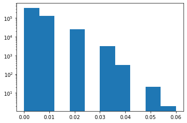
The above example illustrates a signature matrix with very low similarity scores as confirmed by the distribution plot of actual Jaccard similarities.
Example 2#
Suppose we have a signature matrix where all items are similar. We see that across all bands, all the samples are placed in the same buckets. This time, we pass the compute=True flag to cast the dask.bags into a lists as values to the dictionary output of get_buckets.
# some edge case : all items are similar
n = 10
m = 100

# all values are 1
signature = np.full((n, m), 1)

lsh = LSH(signature)
lsh.make_bands(bands=10)
print("Rows per band: ", lsh.r)
print("Number of bands: ", lsh.bands)
display(lsh.get_buckets(compute=True))
Rows per band:  10
Number of bands:  10
{0: [(-4511045881551967787, [0, 1, 2, 3, 4, 5, 6, 7, 8, 9])],
 1: [(-8359770896084742983, [0, 1, 2, 3, 4, 5, 6, 7, 8, 9])],
 2: [(2866674764794135345, [0, 1, 2, 3, 4, 5, 6, 7, 8, 9])],
 3: [(-4164649050109038293, [0, 1, 2, 3, 4, 5, 6, 7, 8, 9])],
 4: [(-4511045881551967787, [0, 1, 2, 3, 4, 5, 6, 7, 8, 9])],
 5: [(-8359770896084742983, [0, 1, 2, 3, 4, 5, 6, 7, 8, 9])],
 6: [(2866674764794135345, [0, 1, 2, 3, 4, 5, 6, 7, 8, 9])],
 7: [(-4164649050109038293, [0, 1, 2, 3, 4, 5, 6, 7, 8, 9])],
 8: [(-4511045881551967787, [0, 1, 2, 3, 4, 5, 6, 7, 8, 9])],
 9: [(-8359770896084742983, [0, 1, 2, 3, 4, 5, 6, 7, 8, 9])]}
Example 3#
Suppose now another signature matrix where there are two groups of sets that are similar. We shall observe that for each band, we have two buckets corresponding to the two similarity groups (1’s group and 2’s group).
# two similar groups
n = 10 # total of 20 samples
m = 100

# concatentate two full matrices: matrix of 1's and 2's
signature = np.concatenate((np.full((n, m), 1), np.full((n, m), 2)))

lsh = LSH(signature)
lsh.make_bands(bands=10)
print("Rows per band: ", lsh.r)
print("Number of bands: ", lsh.bands)
display(lsh.get_buckets(compute=True))
Rows per band:  10
Number of bands:  10
{0: [(2866674764794135345, [0, 1, 2, 3, 4, 5, 6, 7, 8, 9]),
  (-8148071392985430698, [10, 11, 12, 13, 14, 15, 16, 17, 18, 19])],
 1: [(-4164649050109038293, [0, 1, 2, 3, 4, 5, 6, 7, 8, 9]),
  (7929749226918372346, [10, 11, 12, 13, 14, 15, 16, 17, 18, 19])],
 2: [(-4511045881551967787, [0, 1, 2, 3, 4, 5, 6, 7, 8, 9]),
  (499418812276172301, [10, 11, 12, 13, 14, 15, 16, 17, 18, 19])],
 3: [(-8359770896084742983, [0, 1, 2, 3, 4, 5, 6, 7, 8, 9]),
  (5464707384305557384, [10, 11, 12, 13, 14, 15, 16, 17, 18, 19])],
 4: [(2866674764794135345, [0, 1, 2, 3, 4, 5, 6, 7, 8, 9]),
  (-8148071392985430698, [10, 11, 12, 13, 14, 15, 16, 17, 18, 19])],
 5: [(-4164649050109038293, [0, 1, 2, 3, 4, 5, 6, 7, 8, 9]),
  (7929749226918372346, [10, 11, 12, 13, 14, 15, 16, 17, 18, 19])],
 6: [(-4511045881551967787, [0, 1, 2, 3, 4, 5, 6, 7, 8, 9]),
  (499418812276172301, [10, 11, 12, 13, 14, 15, 16, 17, 18, 19])],
 7: [(-8359770896084742983, [0, 1, 2, 3, 4, 5, 6, 7, 8, 9]),
  (5464707384305557384, [10, 11, 12, 13, 14, 15, 16, 17, 18, 19])],
 8: [(2866674764794135345, [0, 1, 2, 3, 4, 5, 6, 7, 8, 9]),
  (-8148071392985430698, [10, 11, 12, 13, 14, 15, 16, 17, 18, 19])],
 9: [(-4164649050109038293, [0, 1, 2, 3, 4, 5, 6, 7, 8, 9]),
  (7929749226918372346, [10, 11, 12, 13, 14, 15, 16, 17, 18, 19])]}