.ipynb .pdf

repository open issue

Binder

Contents

Chapter 8: Winningest Methods in Time Series Forecasting

Compiled by: Sebastian C. Ibañez

In previous sections, we examined several models used in time series forecasting such as ARIMA, VAR, and Exponential Smoothing methods. While the main advantage of traditional statistical methods is their ability to perform more sophisticated inference tasks directly (e.g. hypothesis testing on parameters, causality testing), they usually lack predictive power because of their rigid assumptions. That is not to say that they are necessarily inferior when it comes to forecasting, but rather they are typically used as performance benchmarks.

In this section, we demonstrate several of the fundamental ideas and approaches used in the recently concluded M5 Competition where challengers from all over the world competed in building time series forecasting models for both accuracy and uncertainty prediction tasks. Specifically, we explore the machine learning model that majority of the competition’s winners utilized: LightGBM, a tree-based gradient boosting framework designed for speed and efficiency.

1. M5 Dataset

You can download the M5 dataset from the Kaggle links above.

Let’s load the dataset and examine it.

import numpy as np
import pandas as pd
import matplotlib.pyplot as plt

plot_x_size = 15
plot_y_size = 2

np.set_printoptions(precision = 6, suppress = True)

date_list = [d.strftime('%Y-%m-%d') for d in pd.date_range(start = '2011-01-29', end = '2016-04-24')]

df_calendar = pd.read_csv('../data/m5/calendar.csv')
df_price = pd.read_csv('../data/m5/sell_prices.csv')
df_sales = pd.read_csv('../data/m5/sales_train_validation.csv')

df_sales.rename(columns = dict(zip(df_sales.columns[6:], date_list)), inplace = True)
df_sales

	id	item_id	dept_id	cat_id	store_id	state_id	2011-01-29	2011-01-30	2011-01-31	2011-02-01	...	2016-04-15	2016-04-16	2016-04-17	2016-04-18	2016-04-19	2016-04-20	2016-04-21	2016-04-22	2016-04-23	2016-04-24
0	HOBBIES_1_001_CA_1_validation	HOBBIES_1_001	HOBBIES_1	HOBBIES	CA_1	CA	0	0	0	0	...	1	3	0	1	1	1	3	0	1	1
1	HOBBIES_1_002_CA_1_validation	HOBBIES_1_002	HOBBIES_1	HOBBIES	CA_1	CA	0	0	0	0	...	0	0	0	0	0	1	0	0	0	0
2	HOBBIES_1_003_CA_1_validation	HOBBIES_1_003	HOBBIES_1	HOBBIES	CA_1	CA	0	0	0	0	...	2	1	2	1	1	1	0	1	1	1
3	HOBBIES_1_004_CA_1_validation	HOBBIES_1_004	HOBBIES_1	HOBBIES	CA_1	CA	0	0	0	0	...	1	0	5	4	1	0	1	3	7	2
4	HOBBIES_1_005_CA_1_validation	HOBBIES_1_005	HOBBIES_1	HOBBIES	CA_1	CA	0	0	0	0	...	2	1	1	0	1	1	2	2	2	4
...	...	...	...	...	...	...	...	...	...	...	...	...	...	...	...	...	...	...	...	...	...
30485	FOODS_3_823_WI_3_validation	FOODS_3_823	FOODS_3	FOODS	WI_3	WI	0	0	2	2	...	2	0	0	0	0	0	1	0	0	1
30486	FOODS_3_824_WI_3_validation	FOODS_3_824	FOODS_3	FOODS	WI_3	WI	0	0	0	0	...	0	0	0	0	0	0	0	0	1	0
30487	FOODS_3_825_WI_3_validation	FOODS_3_825	FOODS_3	FOODS	WI_3	WI	0	6	0	2	...	2	1	0	2	0	1	0	0	1	0
30488	FOODS_3_826_WI_3_validation	FOODS_3_826	FOODS_3	FOODS	WI_3	WI	0	0	0	0	...	0	0	1	0	0	1	0	3	1	3
30489	FOODS_3_827_WI_3_validation	FOODS_3_827	FOODS_3	FOODS	WI_3	WI	0	0	0	0	...	0	0	0	0	0	0	0	0	0	0

30490 rows × 1919 columns

df_calendar

	date	wm_yr_wk	weekday	wday	month	year	d	event_name_1	event_type_1	event_name_2	event_type_2	snap_CA	snap_TX	snap_WI
0	2011-01-29	11101	Saturday	1	1	2011	d_1	NaN	NaN	NaN	NaN	0	0	0
1	2011-01-30	11101	Sunday	2	1	2011	d_2	NaN	NaN	NaN	NaN	0	0	0
2	2011-01-31	11101	Monday	3	1	2011	d_3	NaN	NaN	NaN	NaN	0	0	0
3	2011-02-01	11101	Tuesday	4	2	2011	d_4	NaN	NaN	NaN	NaN	1	1	0
4	2011-02-02	11101	Wednesday	5	2	2011	d_5	NaN	NaN	NaN	NaN	1	0	1
...	...	...	...	...	...	...	...	...	...	...	...	...	...	...
1964	2016-06-15	11620	Wednesday	5	6	2016	d_1965	NaN	NaN	NaN	NaN	0	1	1
1965	2016-06-16	11620	Thursday	6	6	2016	d_1966	NaN	NaN	NaN	NaN	0	0	0
1966	2016-06-17	11620	Friday	7	6	2016	d_1967	NaN	NaN	NaN	NaN	0	0	0
1967	2016-06-18	11621	Saturday	1	6	2016	d_1968	NaN	NaN	NaN	NaN	0	0	0
1968	2016-06-19	11621	Sunday	2	6	2016	d_1969	NBAFinalsEnd	Sporting	Father's day	Cultural	0	0	0

1969 rows × 14 columns

df_price

	store_id	item_id	wm_yr_wk	sell_price
0	CA_1	HOBBIES_1_001	11325	9.58
1	CA_1	HOBBIES_1_001	11326	9.58
2	CA_1	HOBBIES_1_001	11327	8.26
3	CA_1	HOBBIES_1_001	11328	8.26
4	CA_1	HOBBIES_1_001	11329	8.26
...	...	...	...	...
6841116	WI_3	FOODS_3_827	11617	1.00
6841117	WI_3	FOODS_3_827	11618	1.00
6841118	WI_3	FOODS_3_827	11619	1.00
6841119	WI_3	FOODS_3_827	11620	1.00
6841120	WI_3	FOODS_3_827	11621	1.00

6841121 rows × 4 columns

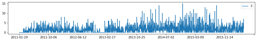
Sample Product

Let’s choose a random product and plot it.

df_sample = df_sales.iloc[3, :]
series_sample = df_sample.iloc[6:]

df_sample

id            HOBBIES_1_004_CA_1_validation
item_id                       HOBBIES_1_004
dept_id                           HOBBIES_1
cat_id                              HOBBIES
store_id                               CA_1
                          ...              
2016-04-20                                0
2016-04-21                                1
2016-04-22                                3
2016-04-23                                7
2016-04-24                                2
Name: 3, Length: 1919, dtype: object

plt.rcParams['figure.figsize'] = [plot_x_size, plot_y_size]

series_sample.plot()
plt.legend()
plt.show()

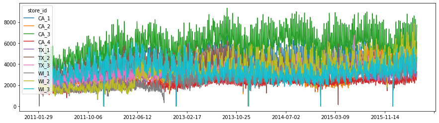
Pick a Time Series

Let’s try and find an interesting time series to forecast.

df_sales_total_by_store = df_sales.groupby(['store_id']).sum()
df_sales_total_by_store

	2011-01-29	2011-01-30	2011-01-31	2011-02-01	2011-02-02	2011-02-03	2011-02-04	2011-02-05	2011-02-06	2011-02-07	...	2016-04-15	2016-04-16	2016-04-17	2016-04-18	2016-04-19	2016-04-20	2016-04-21	2016-04-22	2016-04-23	2016-04-24
store_id
CA_1	4337	4155	2816	3051	2630	3276	3450	5437	4340	3157	...	3982	5437	5954	4345	3793	3722	3709	4387	5577	6113
CA_2	3494	3046	2121	2324	1942	2288	2629	3729	2957	2218	...	4440	5352	5760	3830	3631	3691	3303	4457	5884	6082
CA_3	4739	4827	3785	4232	3817	4369	4703	5456	5581	4912	...	5337	6936	8271	6068	5683	5235	5018	5623	7419	7721
CA_4	1625	1777	1386	1440	1536	1389	1469	1988	1818	1535	...	2496	2839	3047	2809	2677	2500	2458	2628	2954	3271
TX_1	2556	2687	1822	2258	1694	2734	1691	2820	2887	2174	...	3084	3724	4192	3410	3257	2901	2776	3022	3700	4033
TX_2	3852	3937	2731	2954	2492	3439	2588	3772	3657	2932	...	3897	4475	4998	3311	3727	3384	3446	3902	4483	4292
TX_3	3030	3006	2225	2169	1726	2833	1947	2848	2832	2213	...	3819	4261	4519	3147	3938	3315	3380	3691	4083	3957
WI_1	2704	2194	1562	1251	2	2049	2815	3248	1674	1355	...	3862	4862	4812	3236	3069	3242	3324	3991	4772	4874
WI_2	2256	1922	2018	2522	1175	2244	2232	2643	2140	1836	...	6259	5579	5566	4347	4464	4194	4393	4988	5404	5127
WI_3	4038	4198	3317	3211	2132	4590	4486	5991	4850	3240	...	4613	4897	4521	3556	3331	3159	3226	3828	4686	4325

10 rows × 1913 columns

plt.rcParams['figure.figsize'] = [plot_x_size, 4]

df_sales_total_by_store.T.plot()
plt.show()

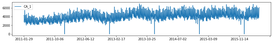
series = df_sales_total_by_store.iloc[0]
print(series.name)
print('Min Dates:' + str(series[series == series.min()].index.to_list()))

plt.rcParams['figure.figsize'] = [plot_x_size, plot_y_size]

series.plot()
plt.legend()
plt.show()

CA_1
Min Dates:['2011-12-25', '2012-12-25', '2013-12-25', '2014-12-25', '2015-12-25']

2. Pre-processing

Before we build a forecasting model, let’s check some properties of our time series.

Is the series non-stationary?

Let’s check.

from statsmodels.tsa.stattools import adfuller

result = adfuller(series)

print('ADF Statistic: %f' % result[0])
print('p-value: %f' % result[1])
print('Critical Values:')

for key, value in result[4].items():
    print('\t%s: %.3f' % (key, value))

ADF Statistic: -2.035408
p-value: 0.271267
Critical Values:
	1%: -3.434
	5%: -2.863
	10%: -2.568

Does differencing make the series stationary?

Let’s check.

def difference(dataset, interval = 1):
    diff = list()
    for i in range(interval, len(dataset)):
        value = dataset[i] - dataset[i - interval]
        diff.append(value)
    return np.array(diff)
 
def inverse_difference(history, yhat, interval=1):
    return yhat + history[-interval]

series_d1 = difference(series)
result = adfuller(series_d1)

print('ADF Statistic: %f' % result[0])
print('p-value: %f' % result[1])
print('Critical Values:')

for key, value in result[4].items():
    print('\t%s: %.3f' % (key, value))

ADF Statistic: -20.626012
p-value: 0.000000
Critical Values:
	1%: -3.434
	5%: -2.863
	10%: -2.568

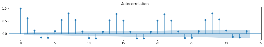
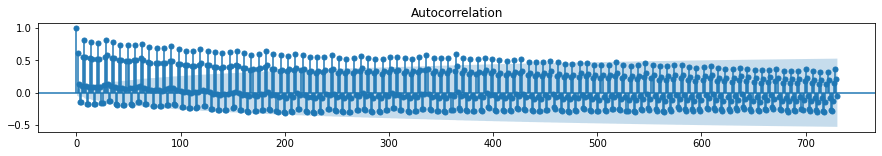
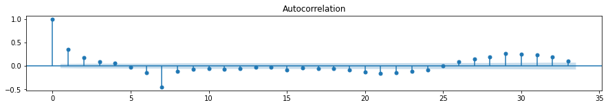
Is the series seasonal?

Let’s check.

from statsmodels.graphics.tsaplots import plot_acf

plt.rcParams['figure.figsize'] = [plot_x_size, plot_y_size]

plot_acf(series)
plt.show()

plot_acf(series, lags = 730, use_vlines = True)
plt.show()

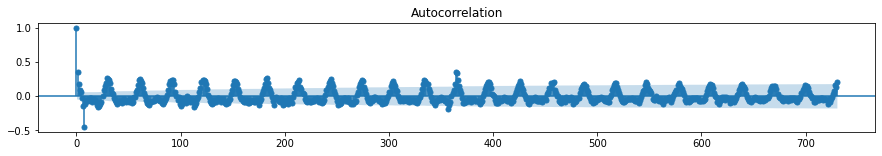
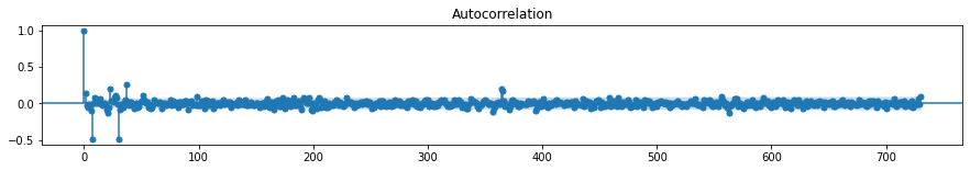
Can we remove the seasonality?

Let’s check.

series_d7 = difference(series, 7)

plt.rcParams['figure.figsize'] = [plot_x_size, plot_y_size]

plot_acf(series_d7)
plt.show()

plot_acf(series_d7, lags = 730, use_vlines = True)
plt.show()

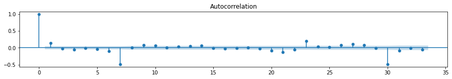
series_d7_d30 = difference(series_d7, 30)

plt.rcParams['figure.figsize'] = [plot_x_size, plot_y_size]

plot_acf(series_d7_d30)
plt.show()

plot_acf(series_d7_d30, lags = 730, use_vlines = True)
plt.show()

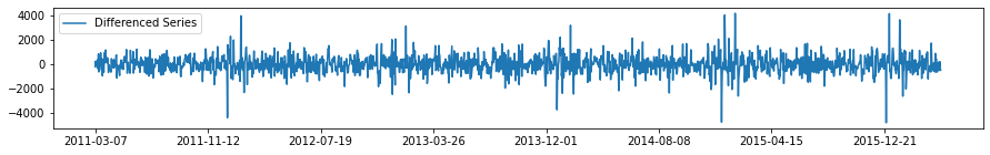
result = adfuller(series_d7_d30)

print('ADF Statistic: %f' % result[0])
print('p-value: %f' % result[1])
print('Critical Values:')

for key, value in result[4].items():
    print('\t%s: %.3f' % (key, value))

ADF Statistic: -8.405429
p-value: 0.000000
Critical Values:
	1%: -3.434
	5%: -2.863
	10%: -2.568

series_d7_d30 = pd.Series(series_d7_d30)
series_d7_d30.index = date_list[37:]

plt.rcParams['figure.figsize'] = [plot_x_size, plot_y_size]

series_d7_d30.plot(label = 'Differenced Series')
plt.legend()
plt.show()

What now?

At this point we have two options:

• Model the seasonally differenced series, then reverse the differencing after making predictions.

• Model the original series directly.

While (vanilla) ARIMA requires a non-stationary and non-seasonal time series, these properties are not necessary for most non-parametric ML models.

3. One-Step Prediction

Let’s build a model for making one-step forecasts.

To do this, we first need to transform the time series data into a supervised learning dataset.

In other words, we need to create a new dataset consisting of \(X\) and \(Y\) variables, where \(X\) refers to the features and \(Y\) refers to the target.

How far do we lookback?

To create the new \((X,Y)\) dataset, we first need to decide what the \(X\) features are.

For the moment, let’s ignore any exogenous variables. In this case, what determines the \(X\)s is how far we lookback. In general, we can treat the lookback as a hyperparameter, which we will call window_size.

Advanced note: Technically, we could build an entire methodology for feature engineering \(X\).

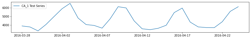
Test Set

To test our model we will use the last 28 days of the series.

### CREATE X,Y ####
def create_xy(series, window_size, prediction_horizon, shuffle = False):
    x = []
    y = []
    for i in range(0, len(series)):
        if len(series[(i + window_size):(i + window_size + prediction_horizon)]) < prediction_horizon:
            break
        x.append(series[i:(i + window_size)])
        y.append(series[(i + window_size):(i + window_size + prediction_horizon)])
    x = np.array(x)
    y = np.array(y)
    return x,y

### HYPERPARAMETERS ###
window_size = 365
prediction_horizon = 1

### TRAIN VAL SPLIT ### (include shuffling later)
test_size = 28
split_time = len(series) - test_size

train_series = series[:split_time]
test_series = series[split_time - window_size:]

train_x, train_y = create_xy(train_series, window_size, prediction_horizon)
test_x, test_y = create_xy(test_series, window_size, prediction_horizon)

train_y = train_y.flatten()
test_y = test_y.flatten()

print(train_x.shape)
print(train_y.shape)
print(test_x.shape)
print(test_y.shape)

(1520, 365)
(1520,)
(28, 365)
(28,)

plt.rcParams['figure.figsize'] = [plot_x_size, plot_y_size]

series[-test_size:].plot(label = 'CA_1 Test Series')
plt.legend()
plt.show()

LightGBM

Now we can build a LightGBM model to forecast our time series.

Gradient boosting is an ensemble method that combines multiple weak models to produce a single strong prediction model. The method involves constructing the model (called a gradient boosting machine) in a serial stage-wise manner by sequentially optimizing a differentiable loss function at each stage. Much like other boosting algorithms, the residual errors are passed to the next weak learner and trained.

For this work, we use LightGBM, a gradient boosting framework designed for speed and efficiency. Specifically, the framework uses tree-based learning algorithms.

To tune the model’s hyperparameters, we use a combination of grid search and repeated k-fold cross validation, with some manual tuning. For more details, see the Hyperparameter Tuning notebook.

Now we train the model on the full dataset and test it.

import lightgbm as lgb

params = {
    'n_estimators': 2000,
    'max_depth': 4,
    'num_leaves': 2**4,
    'learning_rate': 0.1,
    'boosting_type': 'dart'
}

model = lgb.LGBMRegressor(first_metric_only = True, **params)

model.fit(train_x, train_y,
          eval_metric = 'l1', 
          eval_set = [(test_x, test_y)],
          #early_stopping_rounds = 10,
          verbose = 0)

LGBMRegressor(boosting_type='dart', first_metric_only=True, max_depth=4,
              n_estimators=2000, num_leaves=16)

forecast = model.predict(test_x)
s1_naive = series[-29:-1].to_numpy()
s7_naive = series[-35:-7].to_numpy()
s30_naive = series[-56:-28].to_numpy()
s365_naive = series[-364:-336].to_numpy()

print('     Naive MAE: %.4f' % (np.mean(np.abs(s1_naive - test_y))))
print('  s7-Naive MAE: %.4f' % (np.mean(np.abs(s7_naive - test_y))))
print(' s30-Naive MAE: %.4f' % (np.mean(np.abs(s30_naive - test_y))))
print('s365-Naive MAE: %.4f' % (np.mean(np.abs(s365_naive - test_y))))
print('  LightGBM MAE: %.4f' % (np.mean(np.abs(forecast - test_y))))

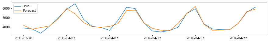
plt.rcParams['figure.figsize'] = [plot_x_size, plot_y_size]

series[-test_size:].plot(label = 'True')
plt.plot(forecast, label = 'Forecast')
plt.legend()
plt.show()

     Naive MAE: 698.0000
  s7-Naive MAE: 372.2857
 s30-Naive MAE: 330.8214
s365-Naive MAE: 247.9286
  LightGBM MAE: 200.5037

Tuning Window Size

How does our metric change as we extend the window size?

from sklearn.model_selection import cross_val_score
from sklearn.model_selection import RepeatedKFold

params = {
    'n_estimators': 2000,
    'max_depth': 4,
    'num_leaves': 2**4,
    'learning_rate': 0.1,
    'boosting_type': 'dart'
}

windows = [7, 30, 180, 365, 545, 730]

results = []
names = []
for w in windows:

    window_size = w

    train_x, train_y = create_xy(train_series, window_size, prediction_horizon)

    train_y = train_y.flatten()

    cv = RepeatedKFold(n_splits = 10, n_repeats = 3, random_state = 123)
    scores = cross_val_score(lgb.LGBMRegressor(**params), train_x, train_y, scoring = 'neg_mean_absolute_error', cv = cv, n_jobs = -1)
    results.append(scores)
    names.append(w)
    print('%3d --- MAE: %.3f (%.3f)' % (w, np.mean(scores), np.std(scores)))

plt.rcParams['figure.figsize'] = [plot_x_size, 5]    
    
plt.boxplot(results, labels = names, showmeans = True)
plt.show()

4. Multi-Step Prediction

Suppose we were interested in forecasting the next \(n\)-days instead of just the next day.

There are several approaches we can take to solve this problem.

### HYPERPARAMETERS ###
window_size = 365
prediction_horizon = 1

### TRAIN VAL SPLIT ###
test_size = 28
split_time = len(series) - test_size

train_series = series[:split_time]
test_series = series[split_time - window_size:]

train_x, train_y = create_xy(train_series, window_size, prediction_horizon)
test_x, test_y = create_xy(test_series, window_size, prediction_horizon)

train_y = train_y.flatten()
test_y = test_y.flatten()

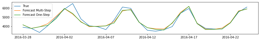
Recursive Forecasting

In recursive forecasting, we first train a one-step model then generate a multi-step forecast by recursively feeding our predictions back into the model.

params = {
    'n_estimators': 2000,
    'max_depth': 4,
    'num_leaves': 2**4,
    'learning_rate': 0.1,
    'boosting_type': 'dart'
}

model = lgb.LGBMRegressor(first_metric_only = True, **params)

model.fit(train_x, train_y,
          eval_metric = 'l1', 
          eval_set = [(test_x, test_y)],
          #early_stopping_rounds = 10,
          verbose = 0)

LGBMRegressor(boosting_type='dart', first_metric_only=True, max_depth=4,
              n_estimators=2000, num_leaves=16)

recursive_x = test_x[0, :]

forecast_ms = []
for i in range(test_x.shape[0]):
    pred = model.predict(recursive_x.reshape((1, recursive_x.shape[0])))
    recursive_x = np.append(recursive_x[1:], pred)
    forecast_ms.append(pred)
    
forecast_ms_rec = np.asarray(forecast_ms).flatten()
forecast_os = model.predict(test_x)

print('  One-Step MAE: %.4f' % (np.mean(np.abs(forecast_os - test_y))))
print('Multi-Step MAE: %.4f' % (np.mean(np.abs(forecast_ms_rec - test_y))))

plt.rcParams['figure.figsize'] = [plot_x_size, plot_y_size]

series[-test_size:].plot(label = 'True')
plt.plot(forecast_ms_rec, label = 'Forecast Multi-Step')
plt.plot(forecast_os, label = 'Forecast One-Step')
plt.legend()
plt.show()

  One-Step MAE: 200.5037
Multi-Step MAE: 214.8020

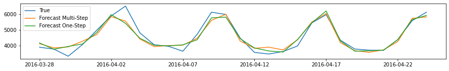
Direct Forecasting

In direct forecasting, we train \(n\) independent models and generate a multi-step forecast by concatenating the \(n\) predictions.

For this implementation, we need to create a new \((X,Y)\) dataset, where \(Y\) is now a vector of \(n\) values.

### HYPERPARAMETERS ###
window_size = 365
prediction_horizon = 28

### TRAIN VAL SPLIT ###
test_size = 28
split_time = len(series) - test_size

train_series = series[:split_time]
test_series = series[split_time - window_size:]

train_x, train_y = create_xy(train_series, window_size, prediction_horizon)
test_x, test_y = create_xy(test_series, window_size, prediction_horizon)

from sklearn.multioutput import MultiOutputRegressor

model = MultiOutputRegressor(lgb.LGBMRegressor(), n_jobs = -1)

model.fit(train_x, train_y)

MultiOutputRegressor(estimator=LGBMRegressor(), n_jobs=-1)

forecast_ms_dir = model.predict(test_x)

print('  One-Step MAE: %.4f' % (np.mean(np.abs(forecast_os - test_y))))
print('Multi-Step MAE: %.4f' % (np.mean(np.abs(forecast_ms_dir - test_y))))

plt.rcParams['figure.figsize'] = [plot_x_size, plot_y_size]

series[-test_size:].plot(label = 'True')
plt.plot(forecast_ms_dir.T, label = 'Forecast Multi-Step')
plt.plot(forecast_os, label = 'Forecast One-Step')
plt.legend()
plt.show()

  One-Step MAE: 200.5037
Multi-Step MAE: 233.6326

Single-Shot Forecasting

In single-shot forecasting, we create a model that attempts to predict all \(n\)-steps simultaneously.

Unfortunately, LightGBM (tree-based methods in general) does not support multi-output models.

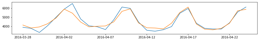
Forecast Combination

An easy way to improve forecast accuracy is to use several different methods on the same time series, and to average the resulting forecasts.

forecast_ms_comb = 0.5*forecast_ms_dir.flatten() + 0.5*forecast_ms_rec

print('  Recursive MAE: %.4f' % (np.mean(np.abs(forecast_ms_rec - test_y))))
print('     Direct MAE: %.4f' % (np.mean(np.abs(forecast_ms_dir - test_y))))
print('Combination MAE: %.4f' % (np.mean(np.abs(forecast_ms_comb - test_y))))

series[-test_size:].plot(label = 'True')
plt.plot(forecast_ms_comb, label = 'Forecast Combination')
plt.show()

  Recursive MAE: 214.8020
     Direct MAE: 233.6326
Combination MAE: 217.0313

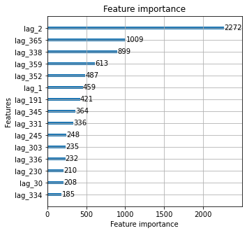
5. Feature Importance

One advantage of GBM models is that it can generate feature importance metrics based on the quality of the splits (or information gain).

### HYPERPARAMETERS ###
window_size = 365
prediction_horizon = 1

### TRAIN VAL SPLIT ###
test_size = 28
split_time = len(series) - test_size

train_series = series[:split_time]
test_series = series[split_time - window_size:]

train_x, train_y = create_xy(train_series, window_size, prediction_horizon)
test_x, test_y = create_xy(test_series, window_size, prediction_horizon)

train_y = train_y.flatten()
test_y = test_y.flatten()
    
params = {
    'n_estimators': 2000,
    'max_depth': 4,
    'num_leaves': 2**4,
    'learning_rate': 0.1,
    'boosting_type': 'dart'
}

model = lgb.LGBMRegressor(first_metric_only = True, **params)

feature_name_list = ['lag_' + str(i+1) for i in range(window_size)]

model.fit(train_x, train_y,
          eval_metric = 'l1', 
          eval_set = [(test_x, test_y)],
          #early_stopping_rounds = 10,
          feature_name = feature_name_list,
          verbose = 0)

LGBMRegressor(boosting_type='dart', first_metric_only=True, max_depth=4,
              n_estimators=2000, num_leaves=16)

plt.rcParams['figure.figsize'] = [5, 5]

lgb.plot_importance(model, max_num_features = 15, importance_type = 'split')
plt.show()

Summary

In summary, this section has shown the following:

• A quick exploration of the M5 dataset and its salient features

• Checking the usual assumptions for classical time series analysis

• Demonstrating the ‘out-of-the-box’ performance of LightGBM models

• Demonstrating how tuning the lookback window can effect forecasting performance

• Demonstrating how tuning the hyperparameters of a LightGBM model can improve performance

• Summarizing the different approaches to multi-step forecasting

• Illustrating that gradient boosting methods can measure feature importance

Many of the methods and approaches shown above are easily extendable. Of note, because of the non-parametric nature of most machine learning models, performing classical inference tasks like hypothesis testing is more challenging. However, trends in ML research have been moving towards greater interpretability of so-called ‘black box’ models, such as SHAP for feature importance and even Bayesian approaches to neural networks for causality inference.

References

[1] S. Makridakis, E. Spiliotis, and V. Assimakopoulos. The M5 Accuracy competition: Results, findings and conlusions. 2020.

[2] S. Makridakis, E. Spiliotis, V. Assimakopoulos, Z. Chen, A. Gaba, I. Tsetlin, and R. Winkler. The M5 Uncertainty competition: Results, findings and conlusions. 2020.

[3] V. Jose, and R. Winkler. Evaluating quantile assessments. Operations research, 2009.

[4] A. Gaba, I. Tsetlin, and R. Winkler. Combining interval forecasts. Decision Analysis, 2017.

Chapter 7: Cross-Correlations, Fourier Transform, and Wavelet Transform Hyperparameter Tuning (Supplementary Notebook)